convolve

named_arrays.convolve(array, kernel, axis=None, where=True, mode='truncate')

Convolve an array with a given \(n\)-dimensional kernel.

Parameters:

• array (ArrayT) – The input array to be convolved. The shape of this array must contain all the axes in axis.

• kernel (KernelT) – The convolution kernel.

• axis (None | str | Sequence[str]) – The logical axes along which to perform the convolution. If None (the default), the convolution will be computed along all the axes of kernel.

• where (bool | AbstractArray) – An optional mask that can be used to exclude elements of array during the convolution operation.

• mode (str) – The method used to extend the array beyond its boundaries. Same options as ndfilters.convolve().

Return type:

ArrayT | KernelT | WhereT

Examples

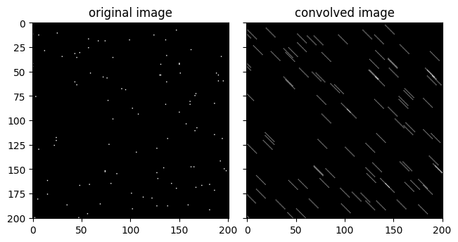
Create a test image and convolve it with an example kernel.

import matplotlib.pyplot as plt
import named_arrays as na

# Define a test image of randomly-positioned
# delta functions
shape_stars = dict(star=101)
index = dict(
    x=na.random.uniform(0, 201, shape_stars).astype(int),
    y=na.random.uniform(0, 201, shape_stars).astype(int),
)
img = na.ScalarArray.zeros(dict(x=201, y=201))
img[index] = 1

# Define an example kernel consisting of a diagonal matrix
kernel = na.arange(0, 10, axis="x") == na.arange(0, 10, axis="y")

# Convolve the test image with the kernel
img_conv = na.convolve(img, kernel)

# Plot the result
fig, axs = plt.subplots(
    ncols=2,
    sharex=True,
    sharey=True,
    constrained_layout=True,
)
axs[0].set_title("original image");
na.plt.imshow(
    X=img,
    axis_x="x",
    axis_y="y",
    ax=axs[0],
    cmap="gray",
);
axs[1].set_title("convolved image");
na.plt.imshow(
    X=img_conv,
    axis_x="x",
    axis_y="y",
    ax=axs[1],
    cmap="gray",
);