Polynomial Fit Function Array Tutorial

A demonstration of creating a function array, fitting a polynomial to it, and then comparing the fit if a different degree polynomial is used.

import numpy as np
import named_arrays as na
import astropy.units as u
import astropy.visualization

astropy.visualization.quantity_support();

Instances of named_arrays.PolynomialFitFunctionArray are defined similarly to named_arrays.FunctionArray by a set of inputs (indepent variables) and outputs (dependent variables), but with the additional parameters coefficient_names (the polynomial terms to fit) and axis_polynomial (the logical axes the polynomial is distributed over). The named_arrays.PolynomialFitFunctionArray.from_degree() classmethod generates the standard coefficient_names for a given polynomial degree over a set of components.

Start by defining a three-dimensional input grid dependent on wavelength, position.x, and position.y.

inputs = na.SpectralPositionalVectorLinearSpace(
    start=na.SpectralPositionalVectorArray(
        wavelength=100 * u.AA,
        position=na.Cartesian2dVectorArray(
            x=-50 * u.arcsec,
            y=-50 * u.arcsec,
        )
    ),
    stop=na.SpectralPositionalVectorArray(
        wavelength=500 * u.AA,
        position=na.Cartesian2dVectorArray(
            x=50 * u.arcsec,
            y=50 * u.arcsec,
        )
    ),
    num=na.SpectralPositionalVectorArray(
        wavelength=2,
        position=na.Cartesian2dVectorArray(
            x=11,
            y=11,
        ),
    ),
    axis=na.SpectralPositionalVectorArray(
        wavelength='wavelength',
        position=na.Cartesian2dVectorArray(
            x='x',
            y='y',
        ),
    ),
)

inputs

SpectralPositionalVectorLinearSpace(
    start=SpectralPositionalVectorArray(
        wavelength=100. Angstrom,
        position=Cartesian2dVectorArray(
            x=-50. arcsec,
            y=-50. arcsec,
        ),
    ),
    stop=SpectralPositionalVectorArray(
        wavelength=500. Angstrom,
        position=Cartesian2dVectorArray(
            x=50. arcsec,
            y=50. arcsec,
        ),
    ),
    axis=SpectralPositionalVectorArray(
        wavelength='wavelength',
        position=Cartesian2dVectorArray(x='x', y='y'),
    ),
    num=SpectralPositionalVectorArray(
        wavelength=2,
        position=Cartesian2dVectorArray(x=11, y=11),
    ),
    endpoint=True,
    centers=False,
)

Using the defined inputs, we calculate a second degree polynomial in outputs.x and outputs.y with 6 total non-zero coefficients. Each x and y has a constant offset, one linear term and one quadratic term. Coefficients c and d depend on both time and wavlength.

t = na.ScalarLinearSpace(-10 * u.s, 10 * u.s, num=3, axis='time')

a = 1 * (u.mm / u.arcsec)
b = .2 * u.mm / (u.arcsec ** 2)
c = t * (u.mm / (u.arcsec * u.s))
d = .001 *  inputs.wavelength * u.mm / (u.AA * u.arcsec ** 2)

outputs = na.Cartesian2dVectorArray(
    x=1 * u.mm + a * inputs.position.x + b * inputs.position.y ** 2 ,
    y=5 * u.mm + c * inputs.position.y + d * inputs.position.x ** 2,
)

Calling named_arrays.PolynomialFitFunctionArray.from_degree() with degree 2, the components position.x and position.y, and two logical axes, "x" and "y", will fit a second degree polynomial to the spatial part of inputs and outputs. The attribute fit.coefficients gives the coefficients of the linear least squares fit to the inputs and outputs. The fit coefficients match those used to create the outputs to machine precision.

fit = na.PolynomialFitFunctionArray.from_degree(
    inputs=inputs,
    outputs=outputs,
    degree=2,
    components=('position.x', 'position.y'),
    axis_polynomial=('x', 'y'),
)

coefficients = fit.coefficients
print(coefficients.components['position.x'].x-a)
print(coefficients.components['position.y*position.y'].x-b)
print(coefficients.components['position.y'].y-c)
print(coefficients.components['position.x*position.x'].y-d)

ScalarArray(
    ndarray=[[0., 0., 0.],
             [0., 0., 0.]] mm / arcsec,
    axes=('wavelength', 'time'),
)
ScalarArray(
    ndarray=[[-5.55111512e-17, -5.55111512e-17, -5.55111512e-17],
             [-5.55111512e-17, -5.55111512e-17, -5.55111512e-17]] mm / arcsec2,
    axes=('wavelength', 'time'),
)
ScalarArray(
    ndarray=[[0., 0., 0.],
             [0., 0., 0.]] mm / arcsec,
    axes=('wavelength', 'time'),
)
ScalarArray(
    ndarray=[[0., 0., 0.],
             [0., 0., 0.]] mm / arcsec2,
    axes=('wavelength', 'time'),
)

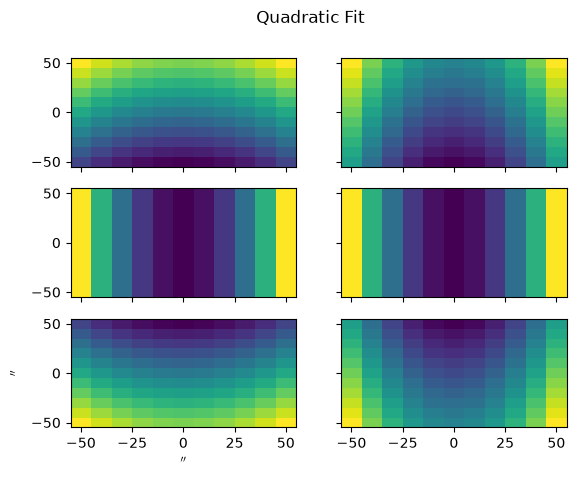
Calling a polynomal function array with a set of inputs uses the fit polynomial to calculate a new set of outputs and returns a named_arrays.FunctionArray with those specfied inputs and calculated outputs. The rms error between the fit and original outputs is low.

best_fit_quad = fit(fit.inputs)
rms_error = np.sqrt(np.square(best_fit_quad.outputs - outputs).sum())
rms_error

Cartesian2dVectorArray(
    x=ScalarArray(
        ndarray=1.11437478e-12 mm,
        axes=(),
    ),
    y=ScalarArray(
        ndarray=4.12849177e-13 mm,
        axes=(),
    ),
)

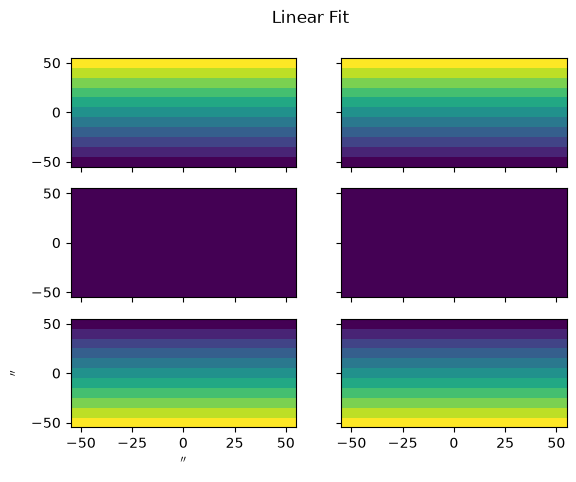
We can also fit a linear function to the original data, and resulting in a much greater error.

fit_linear = na.PolynomialFitFunctionArray.from_degree(
    inputs=inputs,
    outputs=outputs,
    degree=1,
    components=('position.x', 'position.y'),
    axis_polynomial=('x', 'y'),
)
best_fit_linear = fit_linear(fit.inputs)
rms_error = np.sqrt(np.square(best_fit_linear.outputs - outputs).sum())
rms_error

Cartesian2dVectorArray(
    x=ScalarArray(
        ndarray=4759.32768361 mm,
        axes=(),
    ),
    y=ScalarArray(
        ndarray=8580. mm,
        axes=(),
    ),
)

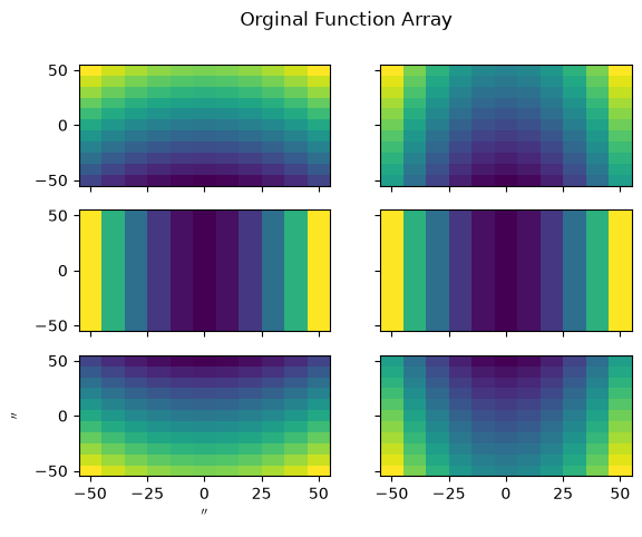
named_arrays plotting routines make it easy to visualize the orginal outputs, and fit outputs, on their inputs grids as a function of wavlength and time.

original_output_y = fit.outputs.y.value
quadratic_fit_output_y = best_fit_quad.outputs.y.value
linear_fit_output_y = best_fit_linear.outputs.y.value

fig, ax = na.plt.subplots(
    axis_cols='wavelength',
    ncols=fit.shape['wavelength'],
    axis_rows='time',
    nrows=fit.shape['time'],
    sharex=True,
    sharey=True
)
na.plt.pcolormesh(
    fit.broadcasted.inputs.position,
    C=original_output_y,
    ax=ax,
)
fig.suptitle('Orginal Function Array');

fig, ax = na.plt.subplots(
    axis_cols='wavelength',
    ncols=fit.shape['wavelength'],
    axis_rows='time',
    nrows=fit.shape['time'],
      sharex=True,
    sharey=True
)
na.plt.pcolormesh(
    fit.broadcasted.inputs.position,
    C=quadratic_fit_output_y,
    ax=ax,
)
fig.suptitle('Quadratic Fit');

fig, ax = na.plt.subplots(
    axis_cols='wavelength',
    ncols=fit.shape['wavelength'],
    axis_rows='time',
    nrows=fit.shape['time'],
    sharex=True,
    sharey=True
)
na.plt.pcolormesh(
    fit.broadcasted.inputs.position,
    C=linear_fit_output_y ,
    ax=ax,
)
fig.suptitle('Linear Fit');

Custom term sets

The set of polynomial terms is given by coefficient_names. from_degree generates the standard set, but you can also build an arbitrary basis: generate the full set, prune the terms you don’t want, and pass the result to the constructor directly.

Here the outputs contain no position.x * position.y cross term, so we can drop it and fit the same data exactly with fewer coefficients.

# `from_degree` generated the full set of degree-2 terms:
print(fit.coefficient_names)

# prune the unused cross term to fit an arbitrary, smaller basis
coefficient_names = [n for n in fit.coefficient_names if n != 'position.x*position.y']

fit_custom = na.PolynomialFitFunctionArray(
    inputs=inputs,
    outputs=outputs,
    coefficient_names=coefficient_names,
    axis_polynomial=('x', 'y'),
)
best_fit_custom = fit_custom(fit.inputs)
rms_error = np.sqrt(np.square(best_fit_custom.outputs - outputs).sum())
print(len(coefficient_names), 'coefficients, rms error =', rms_error)

['', 'position.x', 'position.y', 'position.x*position.x', 'position.x*position.y', 'position.y*position.y']
5 coefficients, rms error = Cartesian2dVectorArray(
    x=ScalarArray(
        ndarray=1.11437478e-12 mm,
        axes=(),
    ),
    y=ScalarArray(
        ndarray=4.12849177e-13 mm,
        axes=(),
    ),
)